Normalizing Transform of a Feature
Let us remark the following proposition which relates the normalizing transform \(\bT_x\) to the feature shape \(\bSigma_x\).
Important
Let \(L\) be an invertible linear transformation in \(\mathbb{R}^2\) whose matrix is denoted by \(\bL\). For any point \(\x\) in the zero-centered unit circle in \(\mathbb{R}^2\), its transformed point by \(L\) is in the ellipse defined by
Note
This note provides a proof of the proposition above.
Fix a point \(\begin{bmatrix} \cos(t) \\ \sin(t) \end{bmatrix}\) of the unit circle in \(\mathbb{R}^2\). We write its transformed point by \(L\) as
Since \(\bL\) is invertible
The squared Euclidean norm of the equality yields
We recognize the equation of an ellipse, which concludes the proof of proposition.
Geometric interpretation of the QR factorization
Consider the shape matrix \(\bSigma_x\). Recall that \(\bSigma_x\) defines the elliptic shape \(\Shape_x\). We want to retrieve the transformation \(L_x\) that satisfies
Observe from the QR factorization \(\bL_x = \bQ \bR\) that \(L_x\) can be decomposed uniquely in two specific transformations \(\bQ\) and \(\bR\). The upper triangular matrix \(\bR\) encodes a transformation that combines of shear and scaling transforms. The orthonormal matrix \(\bQ\) encode a rotation. This geometric interpretation is illustrated in Figure [Geometric interpretation of the QR factorization of linear transform matrix \bL_x.].
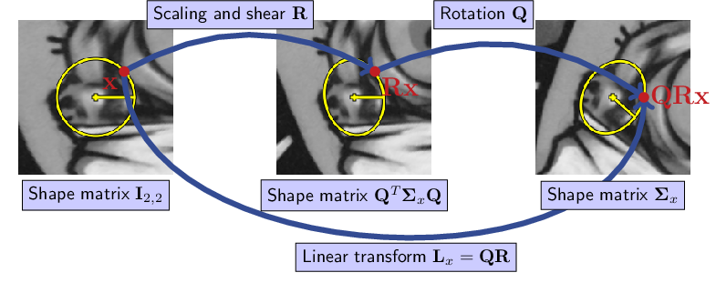
Fig. 4 Geometric interpretation of the QR factorization of linear transform matrix \(\bL_x\).
Unless \(L_x\) involves no rotation, \(\bL_x\) is an upper triangular matrix. Then, because Equation (11) is a Cholesky decomposition, \(\bL_x\) can be identified by unicity of the Cholesky decomposition.
In general, \(\bL_x\) is not upper triangular. Orientations \(\bo_x\) of elliptic shape \(\bSigma_x\) are provided from feature detectors. In SIFT, \(\bo_x\) corresponds to a dominant local gradient orientation.
Thus, introducing \(\theta_x \eqdef \angle \left( \begin{bmatrix}1\\0\end{bmatrix}, \bo_x \right)\), we have
and expanding Equation (11) yields
We recognize the Cholesky decomposition of matrix \(\bQ^T \bSigma_x \bQ\) which is the rotated ellipse as shown in Figure [Geometric interpretation of the QR factorization of linear transform matrix \bL_x.], in which case \(\bL_x\) can be determined completely.
Finally, the affinity that maps the zero-centered unit circle to ellipse \(\Shape_x\) is of the form, in homogeneous coordinates
Calculation of the Normalizing Transform
The algorithm below summarizes how to compute \(\bT_x\).
Important
Calculate the angle
\[\theta_x := \mathrm{atan2}\left( \left\langle \bo_x, \begin{bmatrix}0\\1\end{bmatrix}\right\rangle, \left\langle \bo_x, \begin{bmatrix}1\\0\end{bmatrix}\right\rangle \right)\]Form the rotation matrix
\[\bQ := \begin{bmatrix} \cos(\theta_x) & -\sin(\theta_x) \\ \sin(\theta_x) & \cos(\theta_x) \end{bmatrix}\]Decompose the ellipse matrix \(\bM := \mathrm{Cholesky}(\bQ^T \bSigma_x \bQ)\)
\(\bM\) is a lower triangular matrix such that
- \(\bM \bM^T = \bQ^T \bSigma_x \bQ\)
- \(\bR := (\bM^T)^{-1}\)
- \(\bL := \bQ \bR\)
- \(\bT_x := \begin{bmatrix} \bL & \x \\ \mathbf{0}_2^T & 1 \end{bmatrix}\)