Ellipse Intersections

This section details the implementation of ellipse intersections in Sara. This section is extracted from the appendix of my thesis [Ok:2013:phdthesis] and has been retouched a bit.

[Eberly] provides a comprehensive study on the computation of ellipses intersection, namely the computation of its area and its intersection points. This is non a trivial geometric problem. We complement [Eberly]’s study with additional technical details about the area computation of two intersecting ellipses.

Origin-Centered Axis-Aligned Ellipses

Let \(\mathcal{E}\) be a ellipse with semi-major axis \(a\) and semi-minor axis \(b\), i.e., \(\, a \geq b > 0\). Let us first suppose that \(\mathcal{E}\) is centered at the origin and is axis-aligned oriented, i.e., such that the axis \(a\) is along the \(x\)-axis and the axis \(b\) along the \(y\)-axis. Then,

Important

the equation of ellipse \(\mathcal{E}\) is

(1)\[\frac{x^2}{a^2} + \frac{y^2}{b^2} = 1\]

Ellipse Area

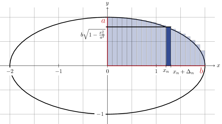
Fig. 1 Riemann sum approximating the upper quadrant area of the ellipse.

Using the symmetry in the ellipse, the area of ellipse \(\mathcal{E}\) is \(4\) times the upper quadrant area of the ellipse, i.e.,

\[\mathop{\mathrm{area}}(\mathcal{E}) = 4 \int_{0}^{a} y(x) \mathop{\mathrm{d}x} = 4 b \int_{0}^{a} \sqrt{1 - \frac{x^2}{a^2}} \mathop{\mathrm{d}x} = \pi a b \]

The integral is the limit of the Riemann sum as illustrated in Figure [Riemann sum approximating the upper quadrant area of the ellipse.].

Let us detail the computation. We use the \(\mathcal{C}^1\)-diffeomorphism change of variable \(\frac{x}{a} = \sin \theta\) which is valid for \([0, a] \rightarrow [0, \pi/2]\). We recall that a \(\mathcal{C}^1\)-diffeomorphism is an invertible differentiable function with continuous derivative.

The differential is \(\mathop{\mathrm{d}x} = a \cos(\theta) \mathop{\mathrm{d}\theta}\) and hence,

Important

\[\begin{aligned} \mathop{\mathrm{area}}(\mathcal{E}) &= 4ab \int_{0}^{\pi/2} \cos^2(\theta) \mathop{\mathrm{d}\theta} \\ &= 4ab \int_{0}^{\pi/2} \frac{1 + \cos(2\theta)}{2} \mathop{\mathrm{d}\theta} \\ &= 4ab \left[ \frac{\theta}{2} + \frac{\sin(2\theta)}{4} \right]_{0}^{\pi/2} \\ &= \pi a b. \end{aligned}\]

Area of an Elliptical Sector

In this part, we review the computation of the area of an ellipse sector. We complement [Eberly] with a bit more details.

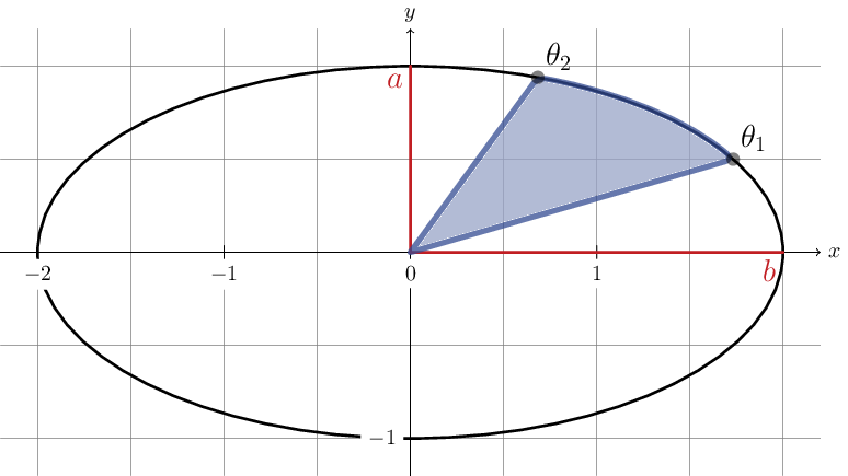
Fig. 2 The ellipse sector delimited by the polar angles \((\theta_1, \theta_2)\) is colored in blue

The elliptic sector area is delimited in polar coordinates by \([\theta_1, \theta_2]\) (with \(\theta_1 < \theta_2\)) as illustrated in Figure [The ellipse sector delimited by the polar angles (\theta_1, \theta_2) is colored in blue]. Using polar coordinates, it equals to the following nonnegative integral

\[A(\theta_1, \theta_2) = \frac{1}{2} \int_{\theta_1}^{\theta_2} r^2 \mathop{\mathrm{d}\theta}.\]

The change of variable in polar coordinates is \(x = r \cos\theta\) and \(y = r \sin\theta\) and, thus with Equation (1), \(\displaystyle\frac{r^2 \cos^2(\theta)}{a^2} + \frac{r^2 \sin^2(\theta)}{b^2} = 1\), therefore

\[\displaystyle r^2 = \frac{a^2 b^2}{b^2 \cos^2(\theta) + a^2 \sin^2(\theta)}.\]

Plugging the formula of \(r\) in the integral,

\[A(\theta_1, \theta_2) = \frac{a^2b^2}{2} \int_{\theta_0}^{\theta_1} \frac{\mathop{\mathrm{d}\theta}}{b^2 \cos^2(\theta) + a^2 \sin^2(\theta)}\]

Now the integrand \(\frac{\mathop{\mathrm{d}\theta}}{b^2 \cos^2(\theta) + a^2 \sin^2(\theta)}\) is invariant by the transformation \(\theta \mapsto \theta+\pi\), i.e.,

\[\frac{\mathop{\mathrm{d}\theta}} {b^2 \cos^2(\theta) + a^2 \sin^2(\theta)} = \frac{\mathop{\mathrm{d}(\theta+\pi)}} {b^2 \cos^2(\theta+\pi) + a^2 \sin^2(\theta+\pi)}.\]

According to Bioche’s rule, a relevant change of variable is the \(\mathcal{C}^1\)-diffeomorphism change of variable \(t = \tan(\theta)\) which is valid for \(]-\pi/2, \pi/2[ \rightarrow ]-\infty, \infty[\). Let us first rewrite

\[\begin{aligned} A(\theta_1, \theta_2) &= \frac{a^2b^2}{2} \int_{\theta_1}^{\theta_2} \frac{\mathop{\mathrm{d}\theta}}{b^2 \cos^2(\theta) + a^2 \sin^2(\theta)}\\ &= \frac{a^2b^2}{2} \int_{\theta_1}^{\theta_2} \frac{\frac{\mathop{\mathrm{d}\theta}}{\cos^2(\theta)}}{b^2 + a^2 \tan^2(\theta)}\\ &= \frac{\cancel{a^2}b^2}{2} \int_{\theta_1}^{\theta_2} \frac{\frac{\mathop{\mathrm{d}\theta}}{\cos^2(\theta)}}{\cancel{a^2} (b/a)^2 + \tan^2(\theta))}\\ \end{aligned}\]

Differentiating \(t=\tan\theta\), \(\mathop{\mathrm{d}t} = \frac{\mathop{\mathrm{d}\theta}}{\cos^2(\theta)}\), thus

\[\begin{aligned} A(\theta_1, \theta_2) &= \frac{b^2}{2} \int_{\tan\theta_1}^{\tan\theta_2} \frac{\mathop{\mathrm{d}t}}{(b/a)^2 + t^2}\\ &= \frac{b^{\cancel{2}}}{2} \left[ \frac{a}{\cancel{b}} \arctan\left(\frac{a}{b} t\right) \right]_{\tan\theta_1}^{\tan\theta_2}\\ &= \frac{ab}{2} \left[ \arctan\left(\frac{a}{b} t\right) \right]_{\tan\theta_1}^{\tan\theta_2} \\ &= \frac{ab}{2} \left( \arctan\left(\frac{a}{b} \tan\theta_2\right) - \arctan\left(\frac{a}{b} \tan\theta_1\right) \right)\end{aligned}\]

Hence,

\[A(\theta_1, \theta_2) = \frac{ab}{2} \left( \arctan\left(\frac{a}{b} \tan\theta_2\right) - \arctan\left(\frac{a}{b} \tan\theta_1\right) \right)\]

Warning

The integral is properly defined for \((\theta_1, \theta_2) \in ]-\pi/2, \pi/2[\). But, using symmetry properties of the ellipse, we can easily retrieve the elliptical sector for any \((\theta_1, \theta_2) \in ]-\pi, \pi[\).

Alternatively, [Eberly] provides a more convenient antiderivative because it is defined in \(]-\pi, \pi]\) as follows

\[F(\theta) = \frac{ab}{2} \left[ \theta - \arctan \left( \frac{(b-a) \sin 2\theta}{(b+a) + (b-a)\cos 2 \theta} \right) \right].\]

Hence, the elliptic sector area equals to the following nonnegative quantity

Important

\[\forall (\theta_1, \theta_2) \in ]-\pi, \pi], \ A(\theta_1, \theta_2) = \left| F(\theta_2) - F(\theta_1) \right|.\]

Area Bounded by a Line Segment and an Elliptical Arc

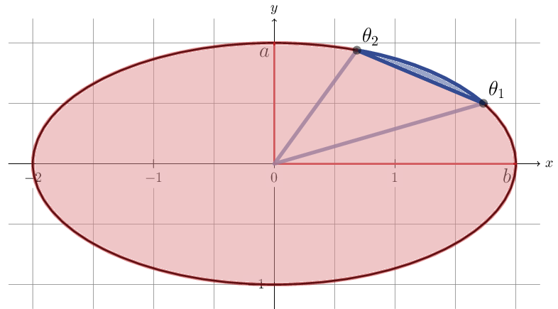
Fig. 3 The ellipse sector bounded by a line segment and the elliptical arc \((\theta_1, \theta_2)\) is colored in blue.

We are interested in computing the elliptic portion by a line segment and the elliptical arc \((\theta_1, \theta_2)\) such that

\[|\theta_2 - \theta_1| \leq \pi \]

This condition is important as a such elliptic portion always corresponds to the blue elliptic portion in Figure [The ellipse sector bounded by a line segment and the elliptical arc (\theta_1, \theta_2) is colored in blue.]. Let us denote the area of such portion by \(B(\theta_1, \theta_2)\). Geometrically, we see that, if \(|\theta_2 - \theta_1| \leq \pi\), then

\[\begin{aligned} B(\theta_1, \theta_2) &= \mathop{\mathrm{area}}(\mathrm{sector(\theta_1, \theta_2)}) - \mathop{\mathrm{area}}(\mathrm{triangle(\theta_1, \theta_2)})\\ &= A(\theta_1, \theta_2) - \frac{1}{2} |x_2y_1 - x_1y_2|\end{aligned}\]

where \((x_i,y_i) = (r_i\cos\theta_i, r_i\sin\theta_i)\) and \(\displaystyle r_i = \frac{ab}{\sqrt{b^2 \cos^2(\theta_i)+a^2 \sin^2(\theta_i)}}\) for \(i \in \{1,2\}\).

Note that the other portion corresponding to the red one in Figure 3 has an area which equals to \(\pi a b - B(\theta_1, \theta_2) \geq B(\theta_1, \theta_2)\) if \(|\theta_2 - \theta_1| \leq \pi\).

To summarize, our portion of interest, illustrated by the blue elliptic portion in Figure 3, has an area which equals to

Important

For any \((\theta_1, \theta_2) \in ]-\pi, \pi]\),

\[\ B(\theta_1, \theta_2) = \left\{ \begin{array}{cl} \displaystyle A(\theta_1, \theta_2) - \frac{1}{2} |x_2y_1 - x_1y_2| & \textrm{if} \ |\theta_2 - \theta_1| \leq \pi \\ \displaystyle \pi a b - A(\theta_1, \theta_2) + \frac{1}{2} |x_2y_1 - x_1y_2| & \textrm{otherwise} \end{array} \right. . \]

General Ellipse Parameterization

The previous sections has provided the basis for area of intersecting ellipses. However, ellipses are neither centered at the origin nor aligned with the axes of the reference frame in general. Therefore, an ellipse \(\mathcal{E}\) is entirely defined by the following geometric information

• a center \(\mathbf{x}_{\mathcal{E}}\),
• axis radii \((a_{\mathcal{E}}, b_{\mathcal{E}})\),
• an orientation \(\theta_{\mathcal{E}}\), i.e., the oriented angle between the \(x\)-axis and the axis of radius \(a_{\mathcal{E}}\).

or more concisely by the pair \((\mathbf{x}_{\mathcal{E}}, \mathbf{\Sigma}_{\mathcal{E}})\) where the positive definite matrix \(\mathbf{\Sigma}_{\mathcal{E}} \in \mathcal{S}^{++}_2\) is such that

(2)\[\mathbf{\Sigma}_{\mathcal{E}} = \mathbf{R}_{\mathcal{E}} \mathbf{D}_{\mathcal{E}} \mathbf{R}_{\mathcal{E}}^T\]

where \(\mathbf{R}_{\mathcal{E}}\) is a rotation matrix defined as

\[\mathbf{R}_{\mathcal{E}} \overset{\textrm{def}}{=} \begin{bmatrix} \cos\theta_{\mathcal{E}} & -\sin\theta_{\mathcal{E}}\\ \sin\theta_{\mathcal{E}} & \cos\theta_{\mathcal{E}} \end{bmatrix}\]

and \(\mathbf{D}_{\mathcal{E}}\) is the diagonal matrix defined as

\[\mathbf{D}_{\mathcal{E}} \overset{\textrm{def}}{=} \begin{bmatrix} 1/b_{\mathcal{E}}^2 & 0\\ 0 & 1/a_{\mathcal{E}}^2 & \\ \end{bmatrix}\]

Note that Equation (2) is the singular value decomposition of \(\mathbf{\Sigma}_{\mathcal{E}}\) if the axis radii satisfy \(a_{\mathcal{E}} \geq b_{\mathcal{E}}\). Thus more generally,

Important

The ellipse \(\mathcal{E}\) is characterized by the equation

\[(\mathbf{x}-\mathbf{x}_{\mathcal{E}})^T \mathbf{\Sigma}_{\mathcal{E}} (\mathbf{x}- \mathbf{x}_{\mathcal{E}}) = 1\]

Or

\[\mathbf{x}^T \mathbf{A}_{\mathcal{E}} \mathbf{x}+ \mathbf{b}_{\mathcal{E}}^T \mathbf{x}+ c_{\mathcal{E}} = 0 \]

where \(\mathbf{A}_{\mathcal{E}} = \mathbf{\Sigma}_{\mathcal{E}}\), \(\mathbf{b}_{\mathcal{E}} = 2 \mathbf{\Sigma}_{\mathcal{E}} \mathbf{x}_{\mathcal{E}}\) and \(c_{\mathcal{E}} = \mathbf{x}_{\mathcal{E}}^T \mathbf{\Sigma}_{\mathcal{E}} \mathbf{x}_{\mathcal{E}} - 1\). Denoting \(\mathbf{x}^T = [x, y]\), ellipse \(\mathcal{E}\) can be defined algebraically as

\[E(x,y) = e_1 x^2 + e_2xy + e_3y^2 + e_4x + e_5y + e_6 = 0, \]

where \(\mathbf{A}_{\mathcal{E}} = \begin{bmatrix} e_1 & e_2/2 \\ e_2/2 & e_3 \end{bmatrix}\), \(\mathbf{b}_{\mathcal{E}}^T = [e_4, e_5]\) and \(c_{\mathcal{E}} = e_6\). This algebraic form is the convenient one that we will use in order to compute the intersection points of two intersecting ellipses.

Intersection Points of Two Ellipses

We explain how we can retrieve the intersection points of two ellipses. Our presentation complements [Eberly].

First let \((\mathcal{E}_i)_{1 \leq i \leq 2}\) be two ellipses defined as

(3)\[(x,y) \in \mathcal{E}_i \iff E_i(x,y) = e_{i1} x^2 + e_{i2} xy + e_{i3} y^2 + e_{i4} x + e_{i5} y + e_{i6} = 0\]

The intersection points of ellipses \((\mathcal{E}_i)_{1 \leq i \leq 2}\) satisfy Equation (3) for \(i \in \{1, 2\}\), i.e., the following equation system holds for intersection points

(4)\[\left\{ \begin{matrix} E_1(x,y) = 0 \\ E_2(x,y) = 0 \end{matrix} \right.\]

Now let us rewrite \(E_i(x,y)\) as a quadratic polynomial in \(x\), i.e.,

\[E_i(x,y) = e_{i1} x^2 + (e_{i2} y + e_{i4}) x + (e_{i3} y^2 + e_{i5} y + e_{i6}) = 0\]

Conveniently we define auxiliary polynomials in \(y\)

\[\begin{aligned} p_0(y) &= e_{13} y^2 + e_{15} y + e_{16} & q_0(y) &= e_{23} y^2 + e_{25} y + e_{26} \\ p_1(y) &= e_{12} y + e_{14} & q_1(y) &= e_{22} y + e_{24} \\ p_2(y) &= e_{11} & q_2(y) &= e_{21} \end{aligned}\]

Introducing the polynomials above, Equation (3) is rewritten as

\[\left\{ \begin{matrix} p_2(y) x^2 + p_1(y) x + p_0(y) = 0 \\ q_2(y) x^2 + q_1(y) x + q_0(y) = 0 \end{matrix} \right.\]

Suppose we know the \(y\)-coordinate of an intersection point, we can calculate the \(x\)-coordinate of this intersection point.

Indeed we multiply the first equation by \(q_2(y)\) and the second equation by \(p_2(y)\).

\[\left\{ \begin{matrix} q_2(y) \times \left( p_2(y) x^2 + p_1(y) x + p_0(y) \right)= 0\times q_2(y)\\ p_2(y) \times \left( q_2(y) x^2 + q_1(y) x + q_0(y) \right)= 0\times p_2(y) \end{matrix} \right.\]

Then subtracting the first equation from the second equation, the monomial \(x^2\) disappears. Thus:

Important

(5)\[x = \frac{p_0(y)q_2(y) - p_2(y)q_0(y)}{p_1(y)q_2(y) - p_2(y)q_1(y)}.\]

Furthermore, Equation (4) is equivalent to the following augmented equation system

\[\left\{ \begin{array}{rl} E_1(x,y) &= 0 \\ x\times E_1(x,y) &= 0 \\ E_2(x,y) &= 0 \\ x\times E_2(x,y) &= 0 \\ \end{array} \right.,\]

And we see more clearly in matrix notation that

Important

\([1, x, x^2, x^3]^T\) is in the nullspace of \(\mathbf{B}(y)\), where \(\mathbf{B}(y)\) is defined as

(6)\[\underbrace{ \begin{bmatrix} p_{0}(y) & p_{1}(y) & p_{2}(y) & 0 \\ 0 & p_{0}(y) & p_{1}(y) & p_{2}(y) \\ q_{0}(y) & q_{1}(y) & q_{2}(y) & 0 \\ 0 & q_{0}(y) & q_{1}(y) & q_{2}(y) \end{bmatrix} }_{\mathbf{B}(y)} \begin{bmatrix} 1 \\ x \\ x^2 \\ x^3 \end{bmatrix} = \begin{bmatrix} 0 \\ 0 \\ 0 \\ 0 \end{bmatrix}\]

We observe that the vector \([1, x, x^2, x^3]^T\) is never zero for any real value \(x\). Thus necessarily the nullspace \(\text{Null}(\mathbf{B}(y))\) is always nontrivial and that means the determinant of \(\mathbf{B}(y)\) has to be zero.

Important

Let the polynomial \(R\) be defined as

\[R \overset{\textrm{def}}{=} \left( p_{0}q_{2} - p_{2}q_{0} \right)^2 - \left( p_{0}q_{1} - p_{1}q_{0} \right) \left( p_{1}q_{2} - p_{2}q_{1} \right),\]

Equation (4) is equivalent to the following quartic equation in \(y\).

(7)\[\det(\mathbf{B}(y)) = R(y) = 0,\]

Using any polynomial solver, we get the \(4\) roots \((y_i)_{1\leq i\leq 4}\) of the quartic polynomial \(R\) and only keep those that are real. Finally \((x_i)_{1\leq i \leq 4}\) are deduced from Equation (5).

Implementation Notes

In Sara, we can use several solvers to retrieve the roots of polynomial \(R\).

1. Companion matrix approach: since Sara depends on Eigen, Eigen has an unsupported Polynomial solver using this simple approach.
2. Jenkins-Traub iterative but very accurate approach also available in Sara.
3. Ferrari’s method available in Sara.

The implementation in Sara uses Ferrari’s method. While more tedious to implement, the method has the advantage of being direct. Also, we experimentally observe Ferrari’s method can sometimes be numerically inaccurate in particular situations where for example one of the ellipse is quasi-degenerate.

In the future, depending on the use case, we can polish the roots to refine the root values.

Intersection Area of Two Ellipses

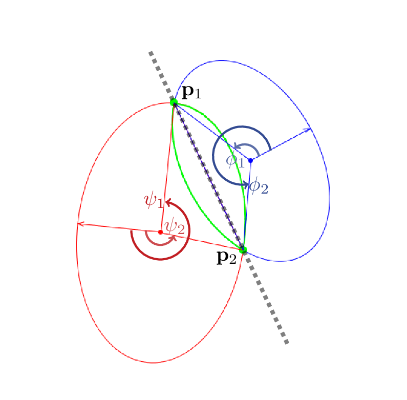
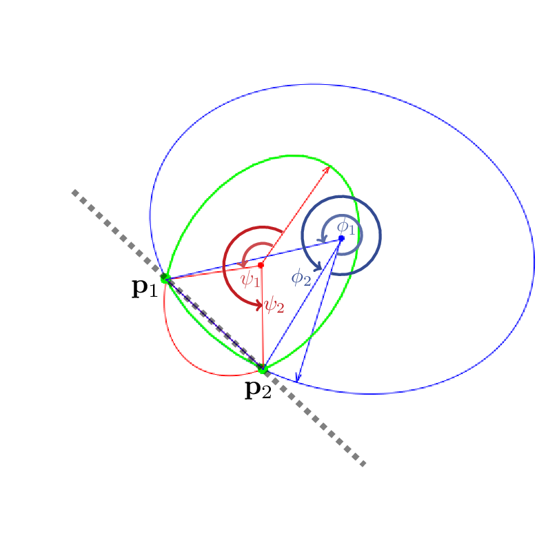
Our presentation complements [Eberly]. In the rest of the section, we consider two ellipses \((\mathcal{E}_i)_{1 \leq i \leq 2}\) and we respectively denote

• the axes of ellipse \(\mathcal{E}_i\) by \((a_i, b_i)\), the ellipse center by \(\mathbf{x}_i\), the orientation by \(\theta_i\), and the direction vectors of axis \(a_i\) and \(b_i\) by

  \[\begin{aligned} \mathbf{u}_i &\overset{\textrm{def}}{=}\begin{bmatrix} \cos(\theta_i) \\ \sin(\theta_i) \end{bmatrix} & \mathbf{v}_i &\overset{\textrm{def}}{=}\begin{bmatrix} -\sin(\theta_i) \\ \cos(\theta_i) \end{bmatrix}\end{aligned}\]

• the area of the elliptic portion bounded a line segment and an arc for ellipse \(\mathcal{E}_i\) by \(B_i\),

• the number of intersection points by \(L\),

• the intersection points by \(\mathbf{p}_i\) for \(i \in \llbracket 1, L \rrbracket\), sorted in a counter-clockwise order, i.e.,

  (8)\[\forall i \in \llbracket 1, L-1\rrbracket,\quad \angle\left([1,0]^T, \mathbf{p}_i\right) \ < \ \angle\left([1,0]^T, \mathbf{p}_{i+1}\right)\]

  where \(\angle(.,.)\) denotes the angle between two vectors in the plane \(\mathbb{R}^2\).

• the polar angles of points \((\mathbf{p}_i)_{1\leq i \leq L}\) with respect to ellipses \(\mathcal{E}_1\) and \(\mathcal{E}_2\) by \((\phi_i)_{1\leq i \leq 2}\) and \((\psi_i)_{1\leq i \leq 2}\), i.e.,

  \[\begin{gathered} \forall i \in \llbracket 1, L\rrbracket, \phi_i \overset{\textrm{def}}{=}\angle\left(\mathbf{u}_1, \mathbf{p}_i - \mathbf{x}_1\right) \\ \forall i \in \llbracket 1, L\rrbracket, \psi_i \overset{\textrm{def}}{=}\angle\left(\mathbf{u}_2, \mathbf{p}_i - \mathbf{x}_2\right)\end{gathered}\]

Retrieving the polar angles

To retrieve the polar angles, we need to place ourselves in the coordinate system \((\mathbf{x}_i, \mathbf{u}_i, \mathbf{v}_i)\). Using the convenient function \(\mathrm{atan2}\) giving values in \(]-\pi,\pi]\), we have

\[\begin{aligned} \phi_i &= \mathrm{atan2} \left( \langle \mathbf{p}_i-\mathbf{x}_1, \mathbf{v}_1 \rangle, \langle \mathbf{p}_i-\mathbf{x}_1, \mathbf{u}_1 \rangle \right)\\ \psi_i &= \mathrm{atan2} \left( \langle \mathbf{p}_i-\mathbf{x}_2, \mathbf{v}_2 \rangle, \langle \mathbf{p}_i-\mathbf{x}_2, \mathbf{u}_2 \rangle \right)\end{aligned}\]

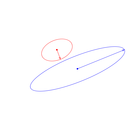
0 or 1 intersection point

Either one ellipse is contained in the other or there are separated as illustrated in Figure [Cases where there is zero or one intersection point.].

Table 1 Cases where there is zero or one intersection point.

An ellipse, say \(\mathcal{E}_1\), is contained in the other \(\mathcal{E}_2\) if and only if its center satisfies \(E_2(\mathbf{x}_1) < 0\). In that case, the area of the intersection is just the area of ellipse \(\mathcal{E}_1\). Otherwise, if there is no containment, the intersection area is zero. In summary,

(9)\[\mathop{\mathrm{area}}(\mathcal{E}_1 \cap \mathcal{E}_2) = \left\{ \begin{array}{ll} \pi a_1 b_1 & \textrm{if}\ E_2(\mathbf{x}_1) < 0\\ \pi a_2 b_2 & \textrm{if}\ E_1(\mathbf{x}_2) < 0\\ 0 & \textrm{otherwise} \end{array} \right.\]

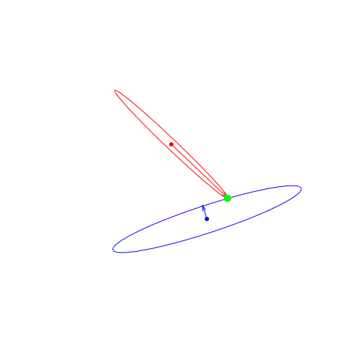
2 intersection points

We will not detail the case when Polynomial (7) have \(2\) roots with multiplicity \(2\). This still corresponds to the case where there are two intersection points. But because of the root multiplicities, one ellipse is contained in the other one and then Equation eq:eq-area01 gives the correct intersection area.

Otherwise, we have to consider two cases as illustrated in Figure [Cases where there are two intersection points.], which [Eberly] apparently forgot to consider. Namely, the cases correspond to whether the center of ellipses \(\mathcal{E}_1\) and \(\mathcal{E}_2\) are on the same side or on opposite side with respect to the line \((\mathbf{p}_1, \mathbf{p}_2)\).

Table 2 Cases where there are two intersection points.

Denoting a unit normal of the line going across the intersection points \((\mathbf{p}_1, \mathbf{p}_2)\) by \(\mathbf{n}\) (cf. Figure 1.9). If the ellipse centers \(\mathbf{x}_1\) and \(\mathbf{x}_2\) are on opposite side with respect to the line \((\mathbf{p}_1, \mathbf{p}_2)\), i.e.,

\[\langle \mathbf{n}, \mathbf{x}_1 - \mathbf{p}_1 \rangle \langle \mathbf{n}, \mathbf{x}_2 - \mathbf{p}_1 \rangle < 0,\]

then

\[\mathop{\mathrm{area}}(\mathcal{E}_1 \cap \mathcal{E}_2) = B_1(\phi_1, \phi_2) + B_2(\psi_1, \psi_2)\]

If they are on the same side with respect to the line \((\mathbf{p}_1, \mathbf{p}_2)\), i.e.,

\[\langle \mathbf{n}, \mathbf{x}_1 - \mathbf{p}_1 \rangle \langle \mathbf{n}, \mathbf{x}_2 - \mathbf{p}_1 \rangle > 0,\]

then

(10)\[\mathop{\mathrm{area}}(\mathcal{E}_1 \cap \mathcal{E}_2) = \left\{ \begin{array}{ll} \displaystyle \left( \pi a_1 b_1 - B_1(\phi_1, \phi_2) \right) + B_2(\psi_1, \psi_2) & \textrm{if} |\langle\mathbf{n},\mathbf{x}_1-\mathbf{p}_1\rangle| \leq |\langle\mathbf{n},\mathbf{x}_2-\mathbf{p}_1\rangle| \\ \\ \displaystyle B_1(\phi_1, \phi_2) + \left( \pi a_2 b_2 - B_2(\psi_1, \psi_2) \right) & \textrm{otherwise}. \end{array} \right.\]

Note that the condition \(|\langle\mathbf{n},\mathbf{x}_1-\mathbf{p}_1\rangle| \leq |\langle\mathbf{n},\mathbf{x}_2-\mathbf{p}_1\rangle|\) in Equation (10) just expresses the fact that the distance of ellipse center \(\mathbf{x}_1\) to the line \((\mathbf{p}_1, \mathbf{p}_2)\) is smaller than the distance of ellipse center \(\mathbf{x}_2\) to the line \((\mathbf{p}_1, \mathbf{p}_2)\).

3 and 4 intersection points

Table 3 Cases where there are three of four intersection points.

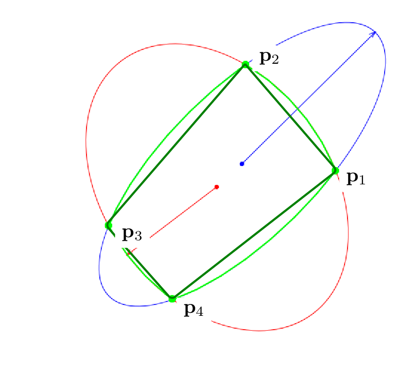
These cases are rather easy to handle. Indeed, we see geometrically from Figure [Cases where there are three of four intersection points.],

\[\mathop{\mathrm{area}}(\mathcal{E}_1 \cap \mathcal{E}_2) = \sum_{i=1}^{L} \underbrace{\min \left( B_1(\phi_i, \phi_{i+1}), B_2(\psi_i, \psi_{i+1}) \right)}_{\textrm{smallest of elliptic portion area}} + \underbrace{\frac{1}{2} \sum_{i=1}^{L} \left| \det\left(\mathbf{p}_i, \mathbf{p}_{i+1}\right) \right|}_{\textrm{area of polygon}\ (\mathbf{p}_1, \mathbf{p}_2, \dots, \mathbf{p}_L)}\]

with \(\phi_{L+1} = \phi_1\), \(\psi_{L+1} = \psi_1\) and \(\mathbf{p}_{L+1} = \mathbf{p}_1\).